DoD programs continue to experience cost overruns; the inadequacies of cost estimation were cited by the Government Accountability Office (GAO) as one of the top problem areas. A recent SEI blog post by my fellow researcher Robert Stoddard, Why Does Software Cost So Much?, explored SEI work that is aimed at improving estimation and management of the costs of software-intensive systems. In this post, I provide an example of how causal learning might be used to identify specific causal factors that are most responsible for escalating costs.

To contain costs, it is essential to understand the factors that drive costs and which ones can be controlled. Although we understand the relationships between certain factors, we do not yet separate the causal influences from non-causal statistical correlations. In Why Does Software Cost So Much?, Robert Stoddard explored how the use of an approach known as causal learning can help the DoD identify factors that actually cause software costs to soar and therefore provide more reliable guidance as to how to intervene to control costs.

Limits of Traditional Cost Estimation

Because it focuses on solely on prediction, traditional cost estimation need not be based on causal knowledge. When prediction is the goal, statistical correlation, regression, and maximum likelihood (ML) estimation methods are suitable for finding predictive associations among data. If the goal, however, is to intervene to deliberately cause a change by changing policies or taking management action, insight into causation is needed.

To control project outcomes, we need to know which factors truly drive those outcomes, as opposed to those merely correlated with them. At the SEI, we have been using causal-modeling tools to evaluate the potential causes of late delivery, cost overruns, and performance gaps. Example causes include the nature of the acquisition environment, number of requirements, team experience, existence of a known feasible architecture early in the project, and more than 100 other factors.

Causal Learning

To identify causes with any certainty, we must move beyond correlation and regression. Although experiments in the form of randomized controlled trials (RCT) are the commonly preferred way of establishing causal relationships, randomization is usually impractical for software costs. Moreover, replication of the software product by multiple teams is far too expensive. We therefore want to establish causation without the expense and challenge of conducting controlled experiments. Establishing causation with observational data remains a vital need and a key technical challenge.

New analytical approaches using directed graphs have arisen to help determine which factors cause which outcomes from observational data. Some approaches use conditional independence tests to reveal the graphical structure of the data. For example, if two variables are independent conditioned on a third, we can conclude that there is no edge connecting them. Other approaches are based on a maximum likelihood score (for example Bayesian information criterion), in which causal edges are incrementally added and removed to search for and improve the score of how well the proposed causal graph fits the data.

In two recent cases studies presented at the International Cost Estimating and Analysis Association (ICEAA), one of which I will discuss in detail here, we used two algorithms, briefly described below, to analyze two datasets. These analyses give insight into the factors for project context, resources, stakeholder dynamics, and level of experience that cause particular project outcomes. From this work, we concluded that causal-modeling methods provide useful and usable insight for project management.

Causal modeling can extend the capabilities available using more traditional statistical methods toward achieving a more fundamental understanding: to identify which of the many options available to a project manager are more likely to have desirable effects on project outcomes. For example, if the project is not progressing well, what interventions should be taken (for example, providing staff with additional training, or reducing the number of difficult requirements or stakeholder decision makers) and what would the effects of those interventions likely be?

A causal understanding of project outcomes and the variables that control them should enable acquisition offices to have the knowledge to

• enhance control of program costs and schedule throughout software development and sustainment lifecycles
• inform "could/should cost" analysis and price negotiations
• improve contract incentives for software-intensive programs
• increase competition using effective criteria related to software cost

Case Study in the Application of Causal Learning

Several years ago, an SEI client from the U.S. Department of Defense (DoD) wanted to study software team dynamics across more than 100 active maintenance projects to better understand what drives software team performance. Although there had been much research published about teams in general and software teams in particular, there was a major gap in any systematic causal research of factors affecting software team performance.

The SEI helped this organization construct a set of surveys that covered a lengthy list of factors mined from Watts Humphrey's publication on leading Team Software Process (TSP) teams. In that book, Humphrey identified more than 120 factors as potential reasons that software teams perform differently. The SEI and the organization measured these factors subjectively through a set of periodic, random surveys to members of the organization's software projects. They then grouped these factors according to the time periods in which change would be expected and managed (see Figure 1 for examples). As such, a set of factors based on a weekly team survey comprised the causal-learning demonstration for this case study.

The study did not purport to cover a complete analysis of this data. Instead, the goal was to show how traditional correlation of data can be misleading to decision makers who wish to act on the analysis and intervene with process improvements expected to increase team performance. We focused on causal discovery of relationships of the independent factors and three outcome factors: cost, schedule, and quality.

We used two causal search algorithms (also known as causal discovery algorithms), focusing on two different types of causal search algorithms that work with discrete data: constraint-based search and score-based search, one algorithm from each causal search-method type:

• PC-Stable, a variant of the constraint-based search algorithm PC, which was among the first to resolve the exponential time barrier for constraint-based causal search of N variables.
• Fast Greedy Equivalence Search (FGES), a score-based search algorithm.

The key difference between this approach and traditional methods is explicitly mapping possible causal paths using graphs, then applying the rules of conditional probability or information theory to determine which paths and edge orientations are most credible. Historically, the problem has been to develop algorithms that could sort through the vast number of possible graphs to find the most credible ones. Applying these algorithms enabled us to make informed inferences about causality and to reduce a complicated problem set to only a few key drivers.

Figure 1 shows the traditional correlation analysis of the independent binary factors against the three ordinal outcome factors. All four correlation measures that we used were in agreement, and significant correlations are marked by the shaded blue cells. As shown, 18 factors were significantly correlated with the quality outcome, five factors were significantly correlated with the cost outcome, and 21 factors were significantly correlated with the schedule outcome.

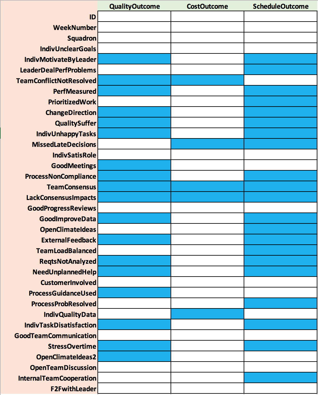
Figure 1: Factors Significantly Correlated with Outcomes

Although not shown, we could also review the correlation among the set of 33 independent factors themselves. Instead, we continued our traditional correlation analysis by performing ordinal logistic regression on each of the outcomes: cost, schedule, and quality. Figure 2 shows that smaller subsets of the factors we originally identified as significant remained significant. Three factors remained significant predicting quality: (1) TeamConsensus, (2) NeedUnplannedHelp, and (3) OpenClimateIdeas2.

In addition, three factors remained significant predicting cost: (1) MissedLateDecisions, (2) TeamConsensus, and (3) ProcessProbResolved. Seven factors remained significant predicting schedule: (1) LeaderDealPerfProblems, (2) PrioritizedWork, (3) MissedLateDecisions, (4) GoodImproveData, (5) GoodTeamCommunication, (6) StressOvertime, and (7) OpenClimateIdeas2. As a result, a decision maker would now be facing a dilemma in terms of which factors to address to improve any one of the outcome factors; and making changes to the wrong ones might offer no or little improvement.

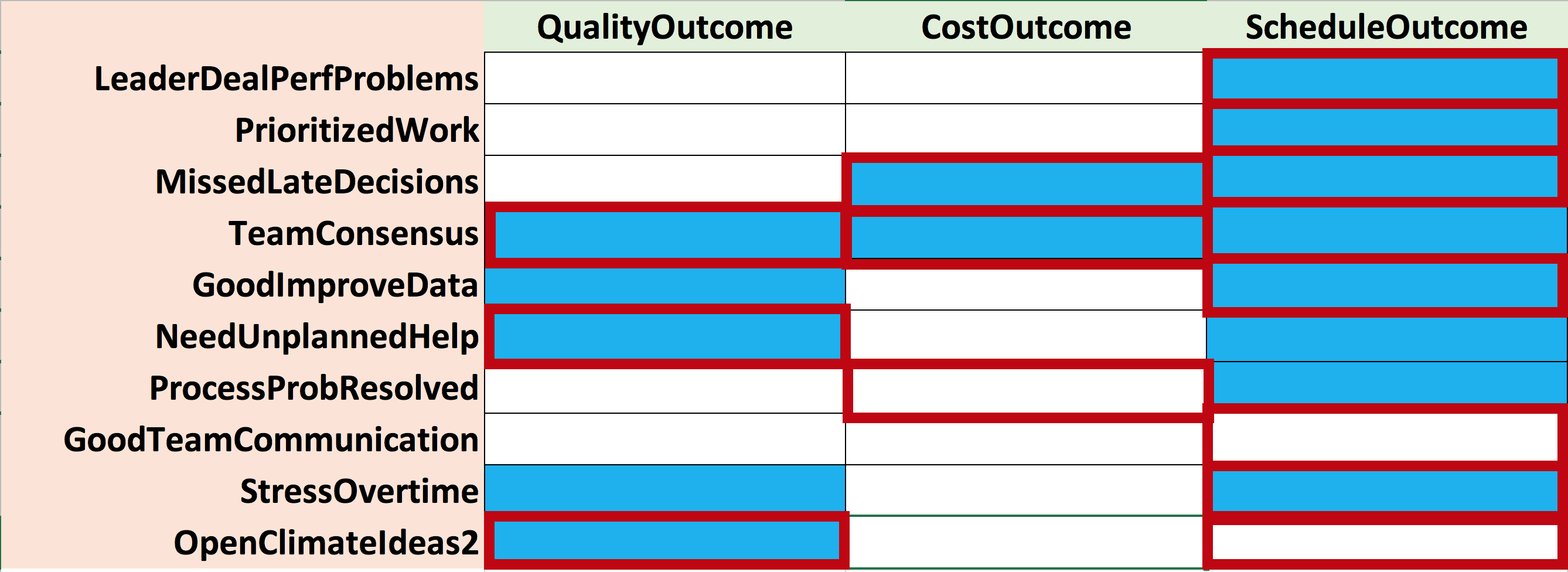
Figure 2: Factors with Red Borders Deemed Significant in Ordinal Logistic Regression

The question arises as to whether searching for the causal relationships and estimating their strength can aid the decision of which actions to take. We therefore initiated two causal-search journeys that serve to show the value that such causal technology could add. Often, we already know something about causation, for example that a cause must precede its effect. Figure 3 displays the knowledge box within the Tetrad tool that specifies known causal constraints used for both discovery searches. The three factors in Tier 1 are purely external and cannot be caused by any other factors in the model. The three factors in Tier 3 represent true outcomes of interest and therefore cannot serve as causal drivers of factors in Tiers 1 and 2.

Figure 3: Tetrad Knowledge Box Used in Discovery for PC-Stable and FGES

Figure 4 shows one of the output displays from Tetrad, the causal structure seen in the search box of Tetrad. This search employed the PC-Stable algorithm. Inferred unmeasured common causation is shown by double arrows, undetermined direction of causation by an edge with no arrows, and direct causation by a directed single arrow.

The causal structure, though hard to read in this graph, shows five factors causally disconnected from the remainder of the factors; and moved to the top. The three outcome factors are highlighted in yellow to distinguish their placement. Although this graph may provide causal answers for any of the possible relationships among factors, we next focused on the key factors of interest.

Figure 5 shows the Markov blanket for the set of three outcome factors using the PC-Stable search algorithm. Only two other factors comprise the Markov blanket: Stress from Overtime (StressOvertime) and Good Improvement Data (GoodImproveData) collected within the team. All influences on the three outcome factors must come through these two factors. In other words, holding these two factors constant, the three outcome factors are independent of all other factors not in the Markov blanket.

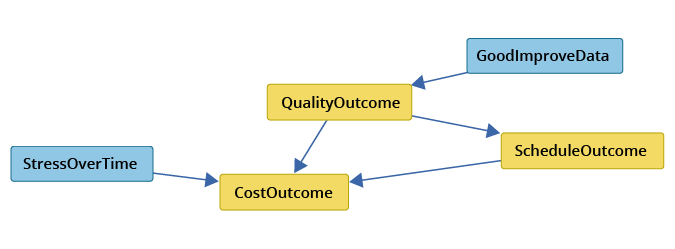
Figure 5: Markov Blanket for Set of Outcome Factors Using PC-Stable

Figure 6 shows how we can also analyze the Markov blanket of any other factor in the causal structure. It shows the Markov blanket for the factor Quality Suffers (QualitySuffer) using the PC-Stable search algorithm. This figure enables us to learn more about how causal influences propagate inward to and outward from Quality Suffers. In particular, Quality Suffers can only influence factors outside of the Markov blanket (such as Cost Outcome) through the factors in the Markov blanket.

Figure 6: Markov Blanket for the QualitySuffer Factor Using PC-Stable

Figure 7 and Figure 8 depict the same results for the Markov blanket of the three outcome factors but using the FGES score-based search algorithm instead of the PC-Stable constraint-based search algorithm. There is agreement in the FGES and PC-Stable results of the Markov blanket for the three outcome factors except that PC-Stable additionally identifies a causal relationship between quality to cost and a causal relationship from Stress from Overtime to cost. The Markov blanket for QualitySuffer agrees between both search algorithms with the exception of the role of two factors: LackConsensusImpacts and IndivUnhappyTasks. Since search algorithms will not necessarily agree, we treat the collective results as input for further study.

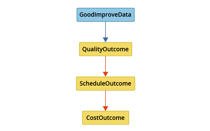
Figure 7: Markov Blanket for Set of Outcome Factors using FGES

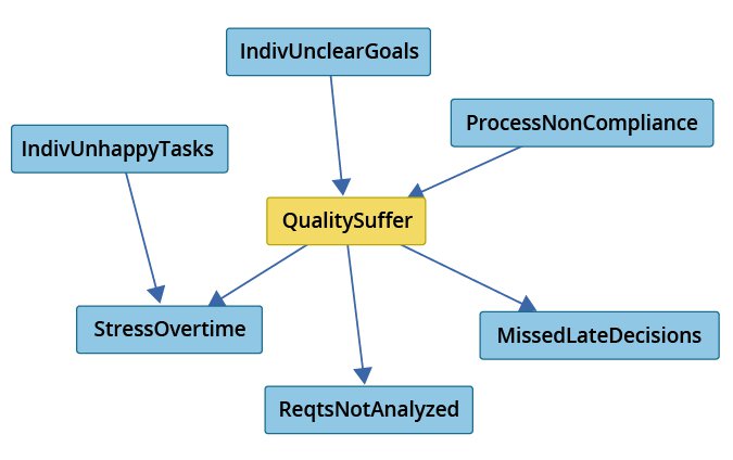
Figure 8: Markov Blanket for the QualitySuffer Factor Using FGES

Both causal searches identified the causal structure among the three outcome factors to be: quality causes schedule causes cost. In the FGES case, quality also had a direct causal influence on cost. Of particular interest is that only two factors directly cause the three outcomes, namely GoodImproveData and StressOvertime. Thus, intervention to improve cost, schedule, and quality outcomes should focus on (1) improving the quality of improvement data collected and used, and (2) taking action to reduce individual stress from working overtime.

What actions one might take to improve the three outcomes can be determined by consulting the causal graph to identify the direct causes of these two factors that might be manipulated to affect their contribution to project outcomes. This focused intervention is in stark contrast to conclusions drawn only from traditional correlation analysis.

Wrapping Up and Looking Ahead

In summary, the analysis presented in this blog posting used causal algorithms to simplify the decision when selecting potential interventions by identifying the two key factors (GoodImprovementData, and StressOvertime) from among actors that could be changed for positive effect on the outcomes. Two separate algorithms produced similar, though not identical results. In addition to providing a few simple predictive relationships, the causal graphs provide more nuanced causal context for interpreting the relationships among variables.

We use this demonstration to argue that software researchers should try these methods on other systems to identify the key controllable factors. Advancing beyond prediction, causal search enables researchers to begin prescribing the nature of actionable interventions that accurately define the expected changes in outcomes.

Our next steps with this work are to

• validate the proposed causal inferences from this study with independent data sets, and
• continue to search for the key controllable factors driving quality, schedule, and cost by applying these techniques to additional data sets.

If readers have software development process and outcome data and would like to participate, please contact us at info@sei.cmu.edu.

Additional Resources

Read Why Does Software Cost So Much? Initial Results from a Causal Search of Project Datasets by Michael Konrad, Robert Stoddard, and Sarah Sheard, presented at the 2018 ICEAA Professional Development & Training Workshop.

Read Robert Stoddard's blog post, Why Does Software Cost So Much?