The Vectors of Code: On Machine Learning for Software

This blog post provides a light technical introduction on machine learning (ML) for problems of computer code, such as detecting malicious executables or vulnerabilities in source code. Code vectors enable ML practitioners to tackle code problems that were previously approachable only with highly-specialized software engineering knowledge. Conversely, code vectors can help software analysts to leverage general, off-the-shelf ML tools without needing to become ML experts.
In this post, I introduce some use cases for ML for code. I also explain why code vectors are necessary and how to construct them. Finally, I touch on current and future challenges in code vector research at the SEI.
Code that learns from code
Here some examples of how ML can learn from source code, executables, and other code representations to make inferences about code:
- Detecting vulnerabilities in source code (Russell et. al., 2018; Sestili et. al., 2018)
- Patching source code (Chen et. al., 2018)
- Judging the maliciousness of an executable (Saxe and Berlin, 2015; Fleshman et. al., 2019)
- Identifying inputs that crash a program, or "fuzzing" (Cheng et. al., 2019)
- Automating reverse engineering (Katz et. al., 2019)
- Detecting design patterns (Zanoni et. al., 2015)
- Naming a function based on its source code (Alon et. al., 2019)
- Generating code based on natural language code descriptions (Yin and Neubig, 2017; Sun et. al., 2019)
These citations are a small fraction of the rapidly-growing body of work on each of the topics above. This paper feed and this "awesome list" are two of the most up-to-date views into the field. The next section introduces some techniques that power ML on code.
Vectors, the currency of machine learning
General-purpose ML algorithms, such as linear models or gradient boosting machines, require the user to input each data point in the form of a numeric vector. This input format means that we need to represent each object of interest as a list of numbers. When using ML to predict corporate revenue, for example, the objects of interest are corporations, and one could begin by defining a length-N vector of a corporation's revenue figures over the previous N months.
The difficulty of defining the relevant numeric data for each object depends on the application. Measuring initial position, velocity, and a few factors related to wind resistance might suffice to estimate the landing position of a projectile. But most ML applications do not have a simple list of rules of physics to dictate what features are relevant. Human-generated objects, such as movies or essays, are medleys of ingenuity and disorganization that intrinsically resist succinct scientific explanation.
When science can't tell us which features are most relevant, a natural strategy is to generate as many features as possible. To create a numeric vector for an essay, one could count every distinct word and character, as well as all the n-grams and n-skip-grams up to some n. However, this strategy leads to extremely long vectors, which can be both computationally cumbersome and statistically inefficient.
Thus, a canonical problem in data analysis is dimension reduction, or how best to fuse a large number of minimally-informative features into far fewer maximally-informative features. In his 1934 psychometrics classic The Vectors of Mind (which motivated the title of this post), Louis Leon Thurstone collected length-60 vectors of personality traits and used factor analysis to reduce this large vector to a smaller vector of length 5 that was sufficient to approximately recover the original length-60 vector. Similarly, modern "personality-to-vector" tools, such as the Myer-Briggs Type Indicator, rely on some form of dimension reduction to summarize a person's responses on a lengthy questionnaire.
Until recently, most methods of dimension reduction (including factor analysis and principal component analysis) were special cases of spectral embeddings, learning the graph structure of a data set by decomposing the matrix of distances or correlations between all pairs of data points or between all pairs of features. Such methods tend not to be scalable, and are typically worse than O(n2) in the number of data points or the number of features, although fast approximate methods exist.
A separate strand of research began to apply neural networks for dimension reduction in the 1980s. Although they approximate spectral embedding methods in special cases, neural network methods are easier to extend with countless exotic architectures for vector embeddings. The simplest kind of neural network embedding, used primarily for pedagogy, is an autoencoder with a single hidden layer:
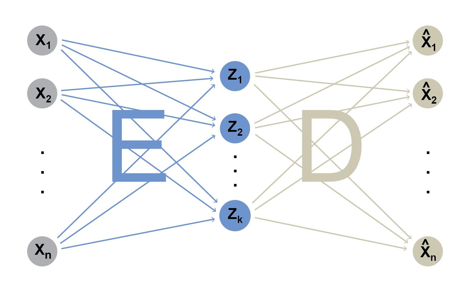
Given a long raw input vector \(x = (x_1, ..., x_n)\), the goal of an autoencoder is to produce a much shorter vector \(z = (z_1, ..., z_k)\) such that the output vector \(\hat x = (\hat x_1, ..., \hat x_n)\) is as similar to the input \(x\) as possible. The arrows pointing to each \(z_j\) on the diagram above represent the weights \(e_{ij}\) in the sum \(z_j := \sum_{i=1}^n e_{ij} x_i\). Similarly, the arrows on the right represent the weighted sum \(\hat x_i := \sum_{i=1}^k d_{ij} z_j\). The weights \(e_{ij}\) can be arranged as an encoding matrix \(E\) and the weights \(d_{ij}\) as a decoding matrix \(D\) such that \(z = x'E\) and \(\hat x = DEx\). If \(\hat x \approx x\), we say that \(z\) successfully encodes \(x\), since we can approximately reconstruct \(x\) from \(z\). Gradient descent (included in any deep learning package) on training examples can lead to approximately-optimal encoder and decoder matrices. This simplest autoencoder can be extended to use a nonlinear link function \(f\) as \(\hat x = D f(Ex)\), include additional hidden layers, or vary the network architecture in myriad other ways.
A drawback of autoencoders is that they fail to capture relationships between objects when applied naively. In natural language processing (NLP) it is often desirable to represent words as numeric vectors. Suppose a corpus contains a vocabulary of 100,000 unique words. If "hello" is the ith word in the vocabulary, the one-hot vector for "hello" is a vector [0, ..., 0, 1, 0, ..., 0] of length 100,000, where the "1" is in the ith position of the vector and all other entries are 0. This vector representation, besides being extremely sparse, provides no information about the relationships between words. Attempting to reduce the dimensionality of these long vectors with an autoencoder would be unhelpful; perhaps the only thing that such an autoencoder would encode is something about the relative frequencies of the k most-frequent words.
The landmark word2vec paper (Mikolov et. al., 2012) introduced one of the first architectures to embed words in a way that capture their relationships]:
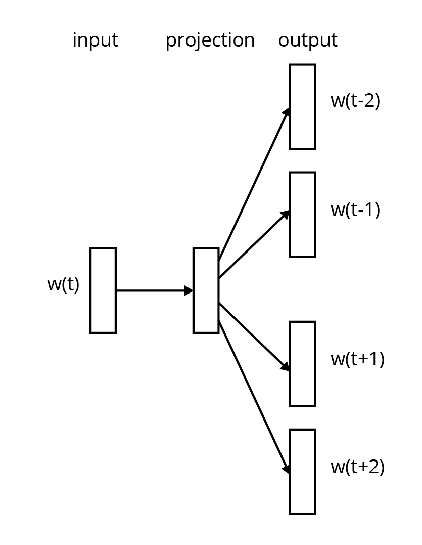
Here the input (left) is a one-hot word vector \(w_t\) that passes through an encoding layer (center), but instead of training the encoder to recover \(w_t\) (on the right, output side), the objective is to recover the nearest neighbors of \(w_t\) across all instances of a word's usages in the training sentences appearing in the corpus. This deceptively simple architecture, trained on billions of word instances, was sufficient to create deeply informative word vectors with as few as 50 elements (on the order of a thousand-fold reduction in length compared to the one-hot vectors).
The general strategy of using encoder-decoder neural networks to embed words (or other objects) is a fertile foundation for generating vectors of code. The next section will identify some potential data inputs for generating such vectors.
The stuff of code
Code is notoriously quirky. Two scripts with the same behavior can look very different. Conversely, two scripts that look very similar can behave in dramatically different ways. The behavior of a script can even depend on the operating system that runs it or the precise flags that were set when compiling it.
These types of problems are not entirely unique to code. ML for code borrows heavily from NLP, where some of the same problems exist in analogous forms. One of the clearest connections between source code and natural language is in their segmentation hierarchies:
| segmentation hierarchy | |
|---|---|
|
natural language |
character → word → sentence → paragraph → document → corpus |
|
source code |
character. → token → line/statement → method → class/file → repository |
Source code differs from natural language in important ways, however. For natural language, word2vec works well in part because closely-related words are often located close together. This is less true for source code because a coding language's grammar is more apt to dictate strong relationships between tokens that are far apart. For example, the opening brace on a lengthly function is connected so strongly to the closing brace that the function becomes entirely uncompilable if either brace goes missing, even when the braces are hundreds of lines apart.
Unlike natural language, which can be at least weakly understood with minimal knowledge of grammar, achieving partial understanding of code requires full understanding of at least some of its grammar. Here is the python grammar, for example. A grammar is a list of production rules. A toy grammar with only two rules illustrates the concept:
- S → SS
- S → Sa
Repeatedly applying the rules in arbitrary order leads to strings of the form "S...Sa....a", and any such string is "valid" by the rules of the grammar. Similarly, iteratively applying the rules of a coding language's grammar according to some trained probability model is one way to produce conceptually plausible synthetic code that is also guaranteed to compile.
Source code and grammar might be the first things that come to mind when we think of code, but there is far more for ML to see.
- Several natural language sources provide clues on the desired meaning and behavior of code: variable names, code documentation, Q&A forums, issue trackers, and version control comments.
- Version control systems provide the edit history of a repository. Modeling this data source may be key to enabling machine-human cooperation in code development (for which syntax highlighting and basic code-completion is a respectable start). Yin et. al. (2018) introduces such a model.
- Compilation pushes source code through a series of compiled representations. Each representation provides a unique window into the structure of the code:
- expanded source code, based on executing macro substitutions
- the abstract syntax tree (AST), which interprets the source code in terms of its grammar, much like sentence diagramming for code
- intermediate representation (IR), various textual representations that the compiler derives from the AST as part of its automatic code optimizations
- assembly language
- a binary executable
- Static program analysis produces several types of code features:
- Alerts of potential code flaws
- Tools like cppdepend can compute interpretable code metrics such as the number of lines in function
- Tools like SciTools Understand can generate a list of instances of (code-entity, relationship, code-entity) tuples such as (Public Method, Define, Variable). Similarly, a control flow graph (CFG) or program dependency graph (PDG) characterizes relationships in code at a more granular level.
- Dynamic program analysis executes code and collects various types of data on what happens as the code runs.
- Source code metadata, including the conventions that a project tries to follow (above and beyond the code grammar). For example, many java projects follow the Spring Model-View-Controller framework, which limits the types of interactions that occur between certain groups of classes.
To our knowledge, no published work attempts to model nearly all of these data sources simultaneously. However, some models have already begun to incorporate more than one source. For example, Sun et. al. (2018) fuses a partial AST, grammar rules, function scope, and a natural language program description as inputs of a single neural network.
Now that we've seen what code is made of, we can ask exactly what are the entities that we would like a code vector to represent. One can specify a code entity in terms of the segmentation levels (perhaps leading to a vector per method or per file) or in terms of stages of the compilation pipeline (perhaps leading to a vector per AST or per executable). The next section highlights models that train vector representations for some of these code entities.
Hidden potential in hidden layers
Chen and Monperrus (2019) review dozens of recent methods for generating code vectors. One of these is code2vec. (Despite its apt name and strong presentation, code2vec is neither the first example of generating code vectors nor the only source for understanding the state of the art.)
Code2vec draws from only two of the many data sources in the stuff of code. It uses the name of each method (as printed in the source code) as the training label in a supervised learning model. The inputs to the model come from randomly sampling paths from the abstract syntax tree (AST) of each method:
- The leaves of an AST refer to tokens (e.g. the words/operators/commands that appear in the source code). The set of tokens over a training corpus determines a token vocabulary.
- A shortest path (excluding the leaves) connects every pair of leaves of the AST. The set of unique paths in a training corpus determines a path vocabulary.
- A path context is a tuple of the form (leaf 1, connecting path, leaf 2).
- The number of path contexts in an AST is O(n^2) where n is the number of leaves, which varies widely across methods. Randomly sampling, say, 200 of these context paths provides a constant-length input for the model.
The code2vec model uses the AST to predict the name of each method. Here is a snapshot of the neural architecture presented in the code2vec paper:
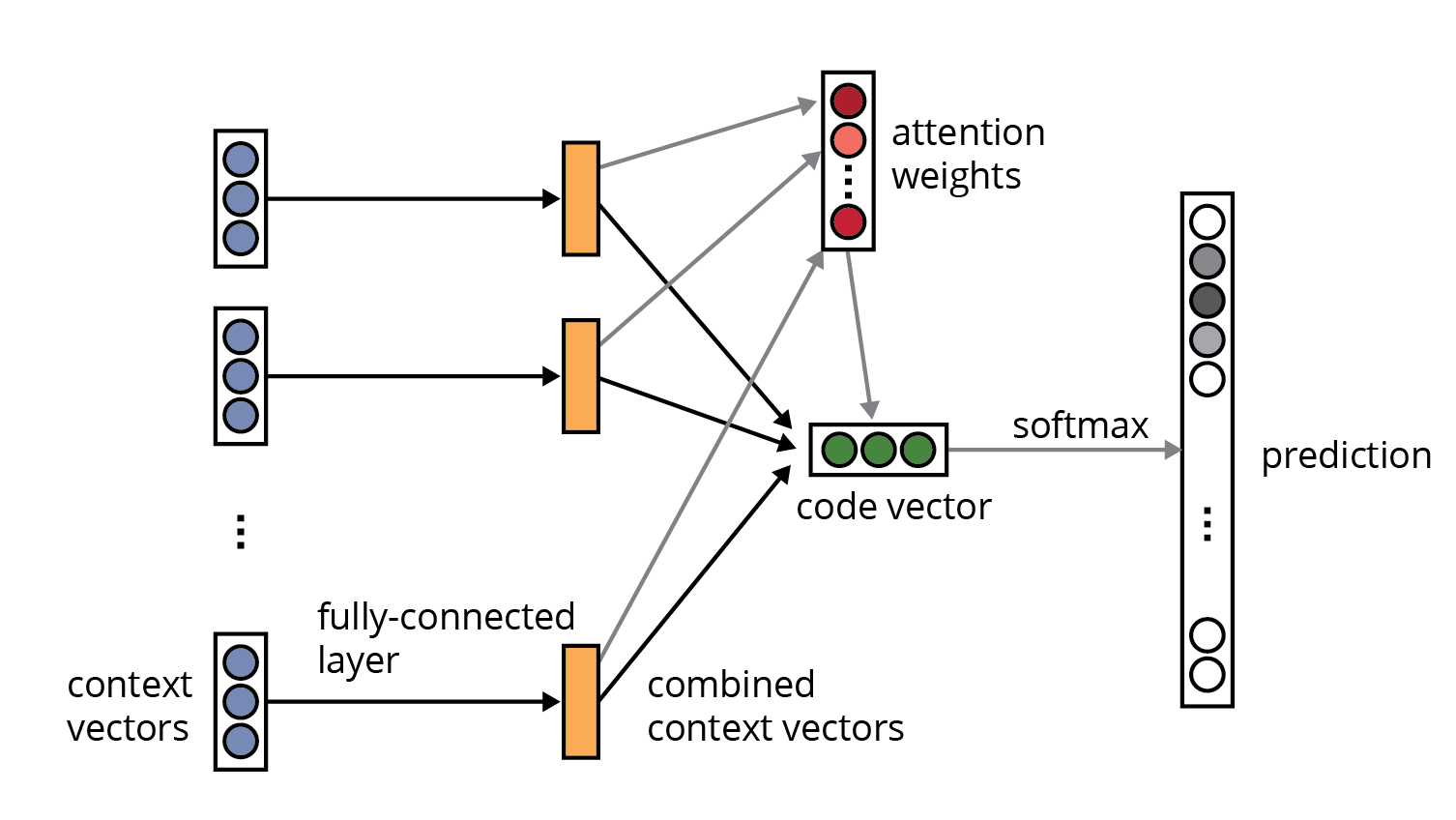
The neural network architecture of code2vec. Source: code2vec: Learning Distributed Representations of Code by Alon et. al., 2018.
This network looks intimidating at first, but much is understandable in terms of the autoencoder example that I presented above. Specifically, each blue circle in the entry nodes of the diagram represents the application of an encoding matrix (such as "E" in the autoencoder). There are two separate encoders in code2vec, one for the tokens vocabulary (with as many rows as there are distinct tokens in the training corpus, on the order of tens of thousands) and one for the paths vocabulary. More concretely, if "foo" is a path context node, the row of the token encoding matrix that corresponds to the index of foo in the token vocabulary represents the vector encoding of foo. We similarly obtain a vector for the other token and the path in the path context containing foo, producing the concatenation of 3 encoding (i.e., 3 blue circles) for each of the 200 input context paths.
The rest of the network is a patchwork of fairly generic neural architecture components, including standard activation functions, densely connected layers, and an attention mechanism. The softmax output layer produces a probability distribution over the method names previously encountered in the training corpus.
Having input a code method to the network, the "code vector" for that method is the activation values of the last hidden layer (colored green). But we could also treat the vector of attention weights as a code vector in its own right. In general, the choice of which part of a network to use for reading off the code vector is not obvious a priori and relies on experimentation or intuition.
A pretrained model such as code2vec is potentially useful even for ML problems that have nothing to do with predicting method names. Given a new method and an AST parser, one can input a sample of the method's context paths to the pretrained model and extract the code vector from the designated hidden layer. The code vector can then function as predictive features in a generic ML algorithm for a new prediction task, saving vast analyst effort by removing the need to build and train a highly customized task-specific neural network.
Code vectors as defined above are not always the most useful features for arbitrary prediction tasks, but the general approach holds great promise. The next section concludes with some application areas where code vectors are gaining relevance at the SEI.
Code vectors at the SEI
Several areas of work at the SEI may soon benefit from the application of code vector methods. These include detecting technical debt artifacts, code repair, detecting false positives in static analysis alerts, and reverse engineering source code from compiled executables, among many other applications.
The SEI's use of ML on code is only getting started. Currently available models incorporate a small fraction of the stuff of code. Future models that intelligently fuse code vectors from more and more-diverse layers of the stuff of code are sure to lead to unprecedented successes in the application of ML to code.
Additional references
Written By

More By The Author
More In Artificial Intelligence Engineering
PUBLISHED IN
Get updates on our latest work.
Sign up to have the latest post sent to your inbox weekly.
Subscribe Get our RSS feedMore In Artificial Intelligence Engineering
Get updates on our latest work.
Each week, our researchers write about the latest in software engineering, cybersecurity and artificial intelligence. Sign up to get the latest post sent to your inbox the day it's published.
Subscribe Get our RSS feed