Imagine that you reverse engineered a piece of malware in painstaking detail only to find that the malware author created a slightly modified version of the malware the next day. You wouldn't want to redo all your hard work. One way to avoid starting over from scratch is to use code comparison techniques to try to identify pairs of functions in the old and new version that are "the same." (I’ve used quotes because “same” in this instance is a bit of a nebulous concept, as we'll see).

Several tools can help in such situations. A very popular commercial tool is zynamics' BinDiff, which is now owned by Google and is free. The SEI's Pharos binary analysis framework also includes a code comparison utility called fn2hash. In this SEI Blog post, the first in a two-part series on hashing, I first explain the challenges of code comparison and present our solution to the problem. I then introduce fuzzy hashing, a new type of hashing algorithm that can perform inexact matching. Finally, I compare the performance of fn2hash and a fuzzy hashing algorithm using a number of experiments.

Background

Exact Hashing

fn2hash employs several types of hashing. The most commonly used is called position independent code (PIC) hashing. To see why PIC hashing is important, we'll start by looking at a naive precursor to PIC hashing: simply hashing the instruction bytes of a function. We'll call this exact hashing.

As an example, I compiled this simple program oo.cpp with g++. Figure 1 shows the beginning of the assembly code for the function myfunc (full code):

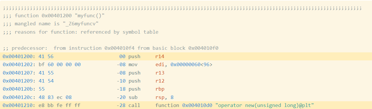
Figure 1: Assembly Code and Bytes from oo.gcc

Exact Bytes

In the first highlighted line of Figure 1, you can see that the first instruction is a push r14, which is encoded by the hexadecimal instruction bytes 41 56. If we collect the encoded instruction bytes for every instruction in the function, we get the following (Figure 2):

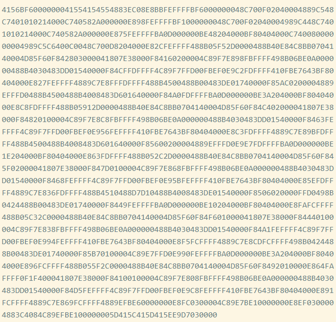
Figure 2: Exact Bytes in oo.gcc

We call this sequence the exact bytes of the function. We can hash these bytes to get an exact hash, 62CE2E852A685A8971AF291244A1283A.

Shortcomings of Exact Hashing

The highlighted call at address 0x401210 is a relative call, which means that the target is specified as an offset from the current instruction (technically, the next instruction). If you look at the instruction bytes for this instruction, it includes the bytes bb fe ff ff, which is 0xfffffebb in little endian form. Interpreted as a signed integer value, this is -325. If we take the address of the next instruction (0x401210 + 5 == 0x401215) and then add -325 to it, we get 0x4010d0, which is the address of operator new, the target of the call. Now we know that bb fe ff ff is an offset from the next instruction. Such offsets are called relative offsets because they are relative to the address of the next instruction.

I created a slightly modified program (oo2.gcc) by adding an empty, unused function before myfunc (Figure 3). You can find the disassembly of myfunc for this executable here.

If we take the exact hash of myfunc in this new executable, we get 05718F65D9AA5176682C6C2D5404CA8D. You’ll notice that's different from the hash for myfunc in the first executable, 62CE2E852A685A8971AF291244A1283A. What happened? Let's look at the disassembly.

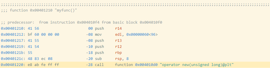
Figure 3: Assembly Code and Bytes from oo2.gcc

Notice that myfunc moved from 0x401200 to 0x401210, which also moved the address of the call instruction from 0x401210 to 0x401220. The call target is specified as an offset from the (next) instruction's address, which changed by 0x10 == 16, so the offset bytes for the call changed from bb fe ff ff (-325) to ab fe ff ff (-341 == -325 - 16). These changes modify the exact bytes as shown in Figure 4.

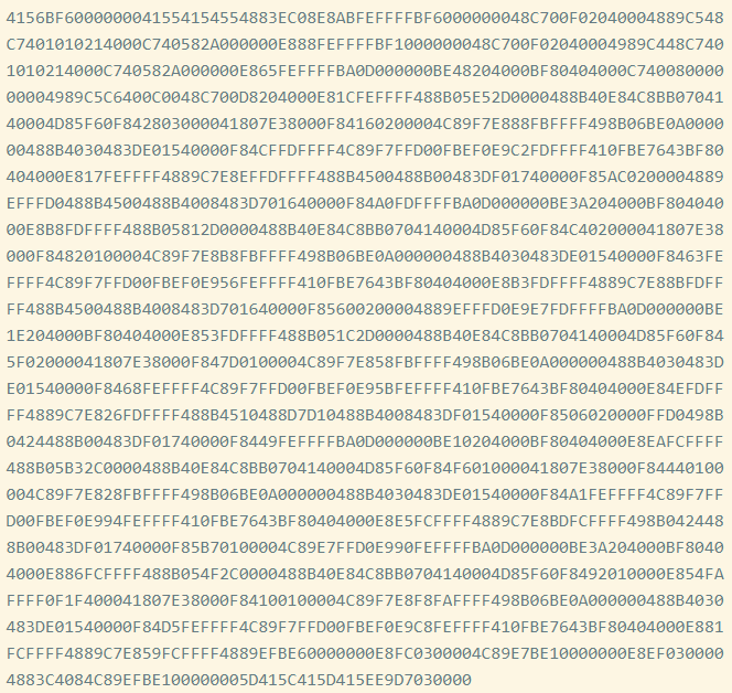
Figure 4: Exact Bytes in oo2.gcc

Figure 5 presents a visual comparison. Red represents bytes that are only in oo.gcc, and green represents bytes in oo2.gcc. The differences are small because the offset is only changing by 0x10, but this is enough to break exact hashing.

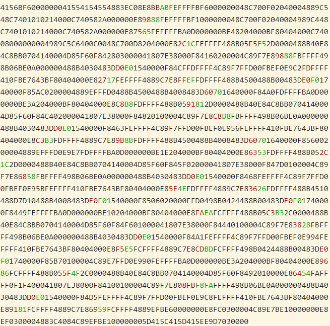
Figure 5: Difference Between Exact Bytes in oo.gcc and oo2.gcc

PIC Hashing

The goal of PIC hashing is to compute a hash or signature of code in a way that preserves the hash when relocating the code. This requirement is important because, as we just saw, modifying a program often results in small changes to addresses and offsets, and we don't want these changes to modify the hash. The intuition behind PIC hashing is very straight-forward: Identify offsets and addresses that are likely to change if the program is recompiled, such as bb fe ff ff, and simply set them to zero before hashing the bytes. That way, if they change because the function is relocated, the function's PIC hash won't change.

The following visual diff (Figure 6) shows the differences between the exact bytes and the PIC bytes on myfunc in oo.gcc. Red represents bytes that are only in the PIC bytes, and green represents the exact bytes. As expected, the first change we can see is the byte sequence bb fe ff ff, which is changed to zeros.

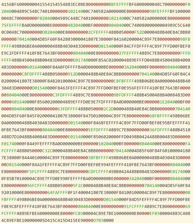
Figure 6: Byte Difference Between PIC Bytes (Red) and Exact Bytes (Green)

If we hash the PIC bytes, we get the PIC hash EA4256ECB85EDCF3F1515EACFA734E17. And, as we would hope, we get the same PIC hash for myfunc in the slightly modified oo2.gcc.

Evaluating the Accuracy of PIC Hashing

The primary motivation behind PIC hashing is to detect identical code that is moved to a different location. But what if two pieces of code are compiled with different compilers or different compiler flags? What if two functions are very similar, but one has a line of code removed? These changes would modify the non-offset bytes that are used in the PIC hash, so it would change the PIC hash of the code. Since we know that PIC hashing will not always work, in this section we discuss how to measure the performance of PIC hashing and compare it to other code comparison techniques.

Before we can define the accuracy of any code comparison technique, we need some ground truth that tells us which functions are equivalent. For this blog post, we use compiler debug symbols to map function addresses to their names. Doing so provides us with a ground truth set of functions and their names. Also, for the purposes of this blog post, we assume that if two functions have the same name, they are "the same." (This, obviously, is not true in general!)

Confusion Matrices

So, let's say we have two similar executables, and we want to evaluate how well PIC hashing can identify equivalent functions across both executables. We start by considering all possible pairs of functions, where each pair contains a function from each executable. This approach is called the Cartesian product between the functions in the first executable and the functions in the second executable. For each function pair, we use the ground truth to determine whether the functions are the same by seeing if they have the same name. We then use PIC hashing to predict whether the functions are the same by computing their hashes and seeing if they are identical. There are two outcomes for each determination, so there are four possibilities in total:

• True positive (TP): PIC hashing correctly predicted the functions are equivalent.
• True negative (TN): PIC hashing correctly predicted the functions are different.
• False positive (FP): PIC hashing incorrectly predicted the functions are equivalent, but they are not.
• False negative (FN): PIC hashing incorrectly predicted the functions are different, but they are equivalent.

To make it a little easier to interpret, we color the good outcomes green and the bad outcomes red. We can represent these in what is called a confusion matrix:

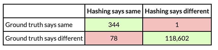
For example, here is a confusion matrix from an experiment in which I use PIC hashing to compare openssl versions 1.1.1w and 1.1.1v when they are both compiled in the same way. These two versions of openssl are quite similar, so we would expect that PIC hashing would do well because a lot of functions will be identical but shifted to different addresses. And, indeed, it does:

Metrics: Accuracy, Precision, and Recall

So, when does PIC hashing work well and when does it not? To answer these questions, we're going to need an easier way to evaluate the quality of a confusion matrix as a single number. At first glance, accuracy seems like the most natural metric, which tells us: How many pairs did hashing predict correctly? This is equal to

For the above example, PIC hashing achieved an accuracy of

You might assume 99.9 percent is pretty good, but if you look closely, there is a subtle problem: Most function pairs are not equivalent. According to the ground truth, there are TP + FN = 344 + 1 = 345 equivalent function pairs, and TN + FP = 118,602 + 78 = 118,680 nonequivalent function pairs. So, if we just guessed that all function pairs were nonequivalent, we would still be right 118680 / (118680 + 345) = 99.9 percent of the time. Since accuracy weights all function pairs equally, it is not the most appropriate metric.

Instead, we want a metric that emphasizes positive results, which in this case are equivalent function pairs. This result is consistent with our goal in reverse engineering, because knowing that two functions are equivalent allows a reverse engineer to transfer knowledge from one executable to another and save time.

Three metrics that focus more on positive cases (i.e., equivalent functions) are precision, recall, and F1 score:

• Precision: Of the function pairs hashing declared equivalent, how many were actually equivalent? This is equal to TP / (TP + FP).
• Recall: Of the equivalent function pairs, how many did hashing correctly declare as equivalent? This is equal to TP / (TP + FN).
• F1 score: This is a single metric that reflects both the precision and recall. Specifically, it is the harmonic mean of the precision and recall, or (2 ∗ Recall ∗ Precision) / (Recall + Precision). Compared to the arithmetic mean, the harmonic mean is more sensitive to low values. This means that if either the precision or recall is low, the F1 score will also be low.

So, looking at the example above, we can compute the precision, recall, and F1 score. The precision is 344 / (344 + 78) = 0.81, the recall is 344 / (344 + 1) = 0.997, and the F1 score is 2 ∗ 0.81 ∗ 0.997 / (0.81 + 0.997) = 0.89. PIC hashing is able to identify 81 percent of equivalent function pairs, and when it does declare a pair is equivalent it is correct 99.7 percent of the time. This corresponds to an F1 score of 0.89 out of 1.0, which is pretty good.

Now, you might be wondering how well PIC hashing performs when there are more substantial differences between executables. Let’s look at another experiment. In this one, I compare an openssl executable compiled with GCC to one compiled with Clang. Because GCC and Clang generate assembly code differently, we would expect there to be a lot more differences.

Here is a confusion matrix from this experiment:

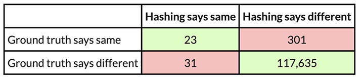
In this example, PIC hashing achieved a recall of 23 / (23 + 301) = 0.07, and a precision of 23 / (23 + 31) = 0.43. So, PIC hashing can only identify 7 percent of equivalent function pairs, but when it does declare a pair is equivalent it is correct 43 percent of the time. This corresponds to an F1 score of 0.12 out of 1.0, which is pretty bad. Imagine that you spent hours reverse engineering the 324 functions in one of the executables only to find that PIC hashing was only able to identify 23 of them in the other executable. So, you would be forced to needlessly reverse engineer the other functions from scratch. Can we do better?

The Great Fuzzy Hashing Debate

In the next post in this series, we will introduce a very different type of hashing called fuzzy hashing, and explore whether it can yield better performance than PIC hashing alone. As with PIC hashing, fuzzy hashing reads a sequence of bytes and produces a hash. Unlike PIC hashing, however, when you compare two fuzzy hashes, you are given a similarity value between 0.0 and 1.0, where 0.0 means completely dissimilar, and 1.0 means completely similar. We will present the results of several experiments that pit PIC hashing and a popular fuzzy hashing algorithm against each other and examine their strengths and weaknesses in the context of malware reverse-engineering.